
This guide explains how to lock only selected cells, rows, columns, or ranges while keeping the rest of the worksheet editable.
-
The Locked setting applies only after you protect the worksheet. Cells marked as Locked stay editable until you enable Protect Sheet.
-
Configure lock and protection settings using the Full Screen Editor.
Recommended approach: unlock everything first
Use this approach when most of the worksheet should remain editable and only specific areas need protection.
Step 1: Unlock the entire worksheet
-
Select the entire worksheet by clicking the triangle in the top-left corner of the sheet, or press Ctrl + A.
-
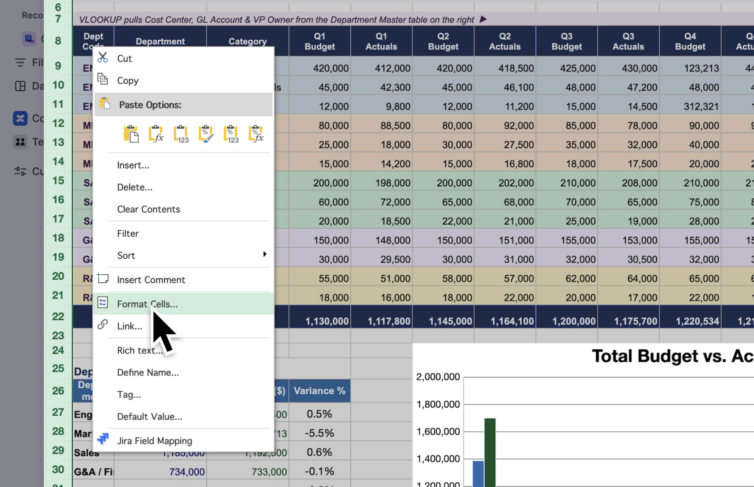
Right-click anywhere in the selected worksheet.
-
Select Format Cells.
-
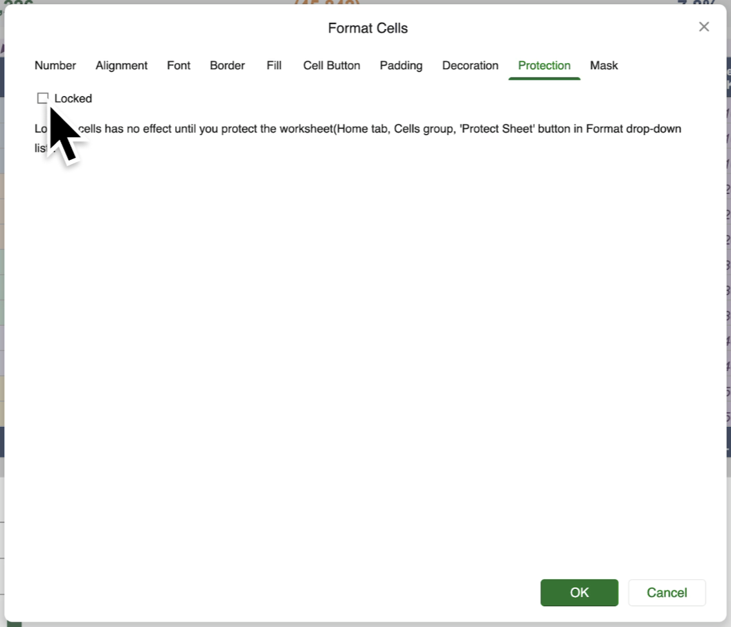
Open the Protection tab.
-
Clear the Locked checkbox.
-
Click OK.
At this stage, all cells are unlocked and will remain editable after sheet protection is enabled.
Step 2: Select what you want to lock
-
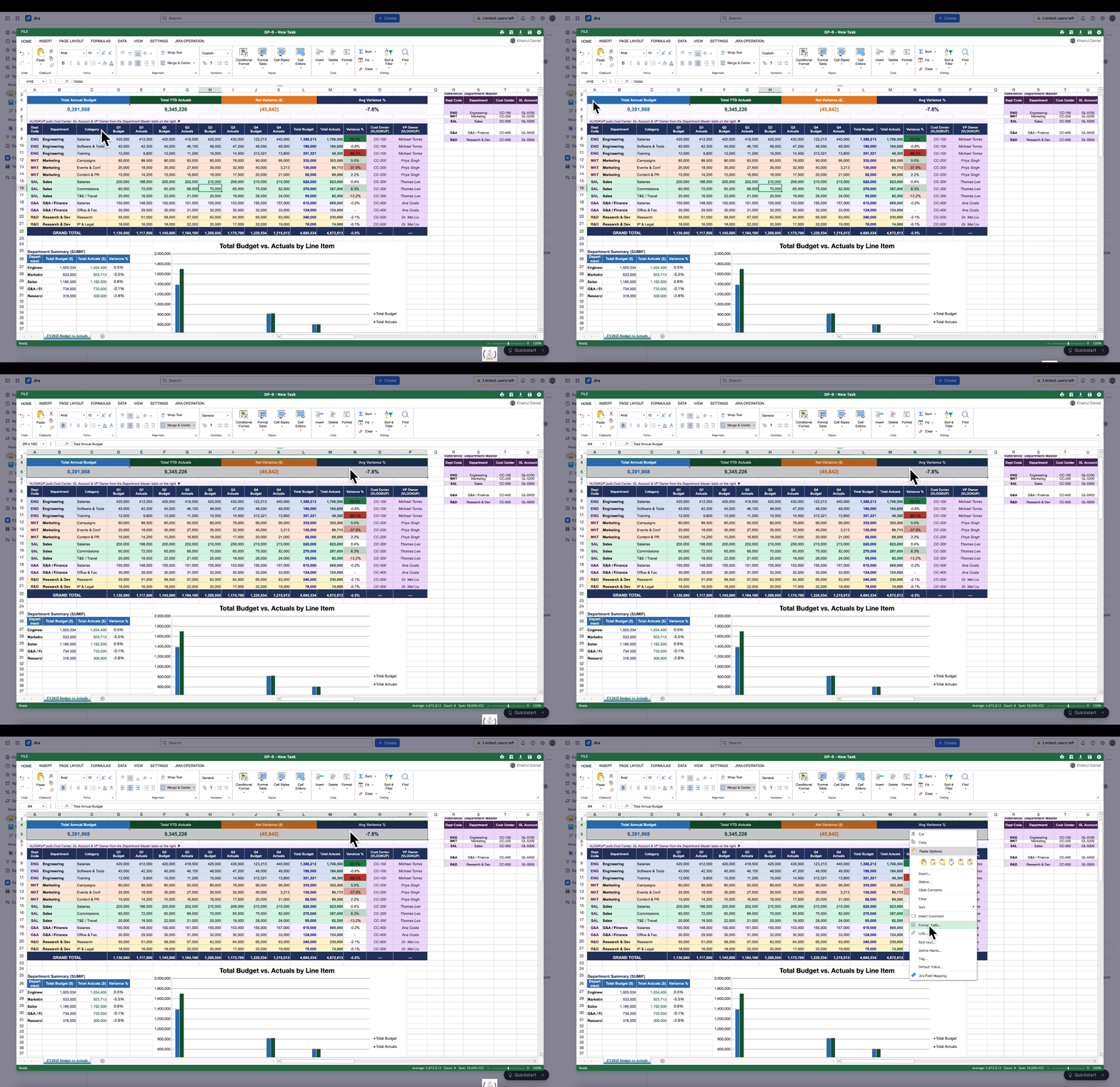
Select the specific cell, range, row, or column that you want to protect.
-
Right-click the selected area.
-
Select Format Cells.
-
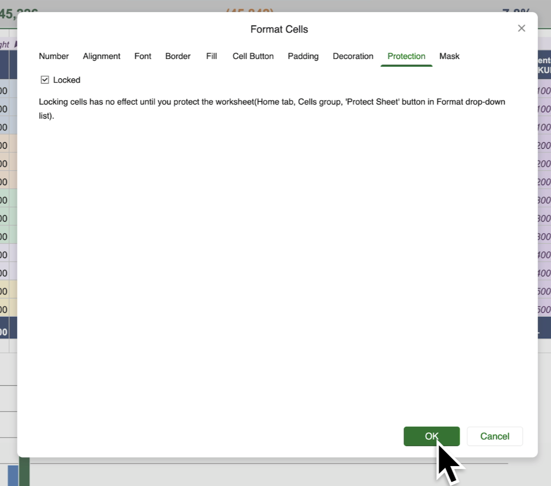
Open the Protection tab.
-
Tick the Locked checkbox.
-
Click OK.
The selected area is now marked as locked, but the lock will only apply after you protect the worksheet.
Step 3: Protect the worksheet
-
Go to the worksheet tab you want to protect.
-
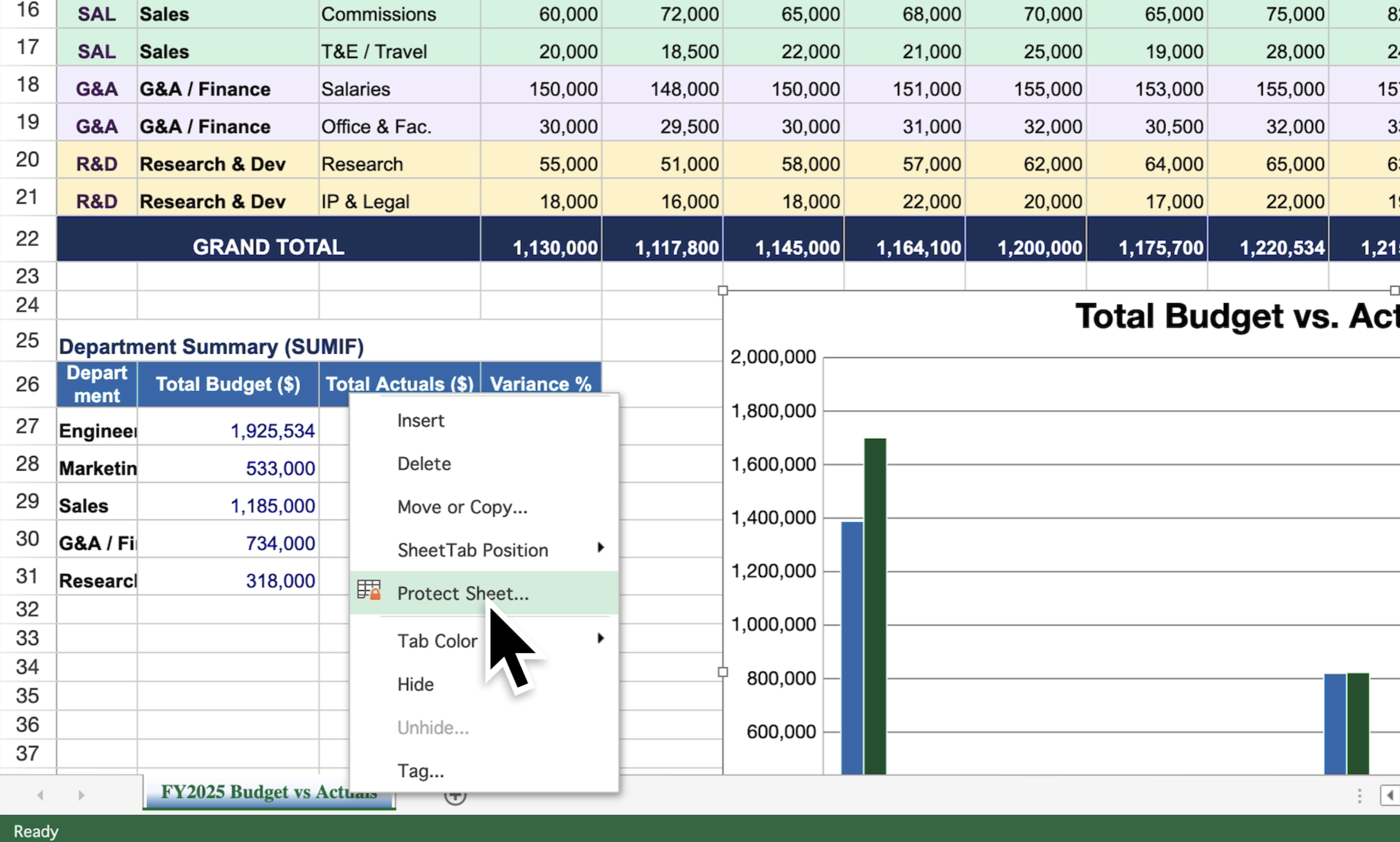
Right-click the worksheet tab and select Protect Sheet.
-
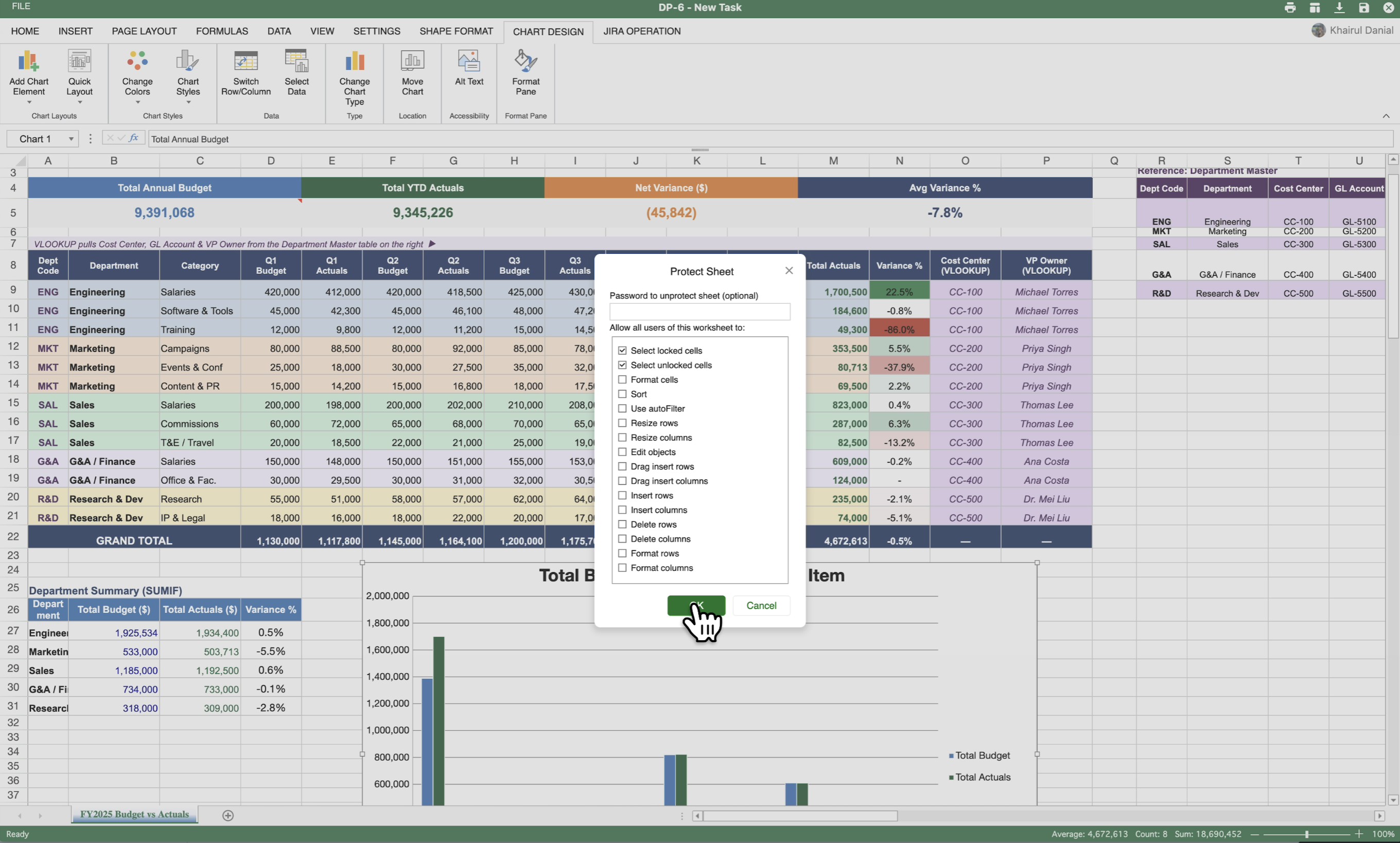
Choose which actions users are allowed to perform while the sheet is protected.
-
Optional: enter a password to prevent users from removing the protection.
-
Click OK.
Result: Users can edit only unlocked cells. Locked cells, rows, columns, or ranges cannot be edited.
Quick example
For example, suppose your worksheet contains:
-
Row 1: Headers
-
Rows 2–20: User input fields
-
Column F: Formulas
To protect the important areas while still allowing users to enter data:
-
Unlock the entire worksheet.
-
Lock Row 1.
-
Lock the formula cells in Column F.
-
Protect the worksheet with a password.
Result: Users can edit rows 2–20, while the headers and formula cells remain protected.
Alternative method: lock only a selected area
If the rest of the worksheet is already unlocked, you can lock only the area you need:
-
Select the cell, range, row, or column you want to lock.
-
Right-click the selection and choose Format Cells.
-
Open the Protection tab.
-
Tick Locked.
-
Click OK.
-
Right-click the worksheet tab and select Protect Sheet.
Best practices
-
Unlock the worksheet first, then lock only the cells that need protection.
-
Use clear labels, instructions, or formatting so users know which cells they can edit.
-
Use a password when you need to prevent users from removing sheet protection.
-
Test the worksheet after protecting it to confirm that only the intended cells remain editable.